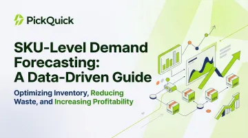
Introduction
Many regional FMCG brands struggle with a critical blind spot: they track overall category sales but miss the individual product variants that drive revenue. SKU-level demand forecasting is the practice of predicting future sales volumes for each individual product variant—by size, flavor, weight, or pack—rather than at a category or brand aggregate level.
This granularity matters in Quick Commerce. When a single SKU goes out of stock on Blinkit or Zepto, shoppers see it immediately. The result? Direct lost revenue, poor availability scores, and damaged search rankings. Both platforms prioritize search rankings based on fill rates, meaning brands that repeatedly fall short during demand spikes face algorithmic deprioritization.
Getting SKU forecasting right is what separates brands that consistently hold shelf position from those that bleed ranking points every time demand spikes.
Key Takeaways
- SKU-level forecasting predicts demand for each product variant separately, not aggregated by brand or category
- In Quick Commerce, forecast errors create immediate stockouts or dark store overstock—both carry measurable costs
- Inputs include historical sales, seasonal patterns, promotional calendars, and platform-specific signals like search ranking and visibility
- Models range from time series baselines to machine learning approaches that factor in external events — promotions, festivals, price changes
- Accurate forecasting directly improves replenishment cycles, in-stock rates, and how platforms rank your SKUs
What Is SKU-Level Demand Forecasting?
SKU-level demand forecasting is the process of generating separate demand predictions for each Stock Keeping Unit, treating each variant—such as a 500g pack versus a 1kg pack of the same masala—as a distinct entity with its own demand behavior.
The outcome this process delivers is precise: aligning inventory to actual consumption patterns at the most granular level, so replenishment decisions are driven by data rather than intuition or blanket category averages.
How it differs from aggregate forecasting:
Category-level or brand-level forecasts can show healthy overall demand while a critical SKU is consistently stocked out. SKU-level forecasting surfaces these hidden imbalances that category-level views miss.
Take a masala brand with strong aggregate sales: the 100g Biryani Masala pack could be perpetually out of stock while the 200g Chaat Masala variant sits idle in the dark store. Aggregate numbers would never flag this.
The two approaches serve different purposes:
| Forecast Type | Primary Use |
|---|---|
| Aggregate (category/brand) | Procurement budgets and financial planning |
| SKU-level | Replenishment orders, shelf allocation, dark store assortment |
Why SKU-Level Forecasting Is Critical in Quick Commerce
The Structural Reality of Dark Stores
Quick Commerce amplifies forecasting stakes because dark stores carry a limited, curated SKU assortment with no backroom buffer. QC dark stores operate within 2,000–4,000 sq. ft., capping assortments at 2,000–5,000 SKUs, compared to 10,000+ in modern supermarkets. Every out-of-stock event is visible in real time on the app and affects conversion, ratings, and platform-assigned visibility.
The cost of getting it wrong:
A mid-performing creator post driving 3,000 visits to Blinkit over a 6-hour spike with a 40% out-of-stock rate results in approximately ₹25,920 in lost GMV from a single post in a single day. Multiply that across dozens of SKUs and multiple cities, and the revenue leakage becomes severe.
Platform-Specific Demand Fragmentation
The same SKU can show completely different velocity patterns across platforms and pin codes. Masala brands, for instance, see distinct behaviors:
- Blinkit: Strong blended masala performance with high search volume
- Zepto: Stable demand once listed, but difficult initial onboarding
- Swiggy Instamart: Best masala platform in India with highest variety acceptance
- JioMart: Bulk pack sizes with monthly purchasing patterns
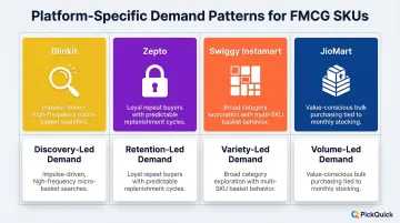
Regional brands operating without SKU-level forecasting on QC platforms face dangerous demand fragmentation that aggregate forecasts cannot capture.
Compressed Replenishment Cycles
Unlike traditional retail with weekly or biweekly restocking, QC dark stores require daily or near-daily replenishment decisions. FMCG majors have reworked urban replenishment cycles to support multiple restocks a day in high-density zones.
This compression means forecast errors compound rapidly rather than self-correcting over a longer cycle. A 20% forecast error that might be absorbed over a two-week retail cycle becomes a same-day stockout in Quick Commerce. That cycle compression also exposes a second structural problem: offline demand data offers almost no predictive value for QC.
Offline Demand Doesn't Translate
For regional FMCG and food brands with strong offline presence, QC demand patterns diverge from GT/MT patterns due to different shopper profiles, basket sizes, and purchase occasions.
The behavioral split is stark: QC shoppers buy smaller packs more frequently for immediate consumption. Modern trade shoppers buy larger packs occasionally for pantry stocking. Porting offline forecasts directly to QC creates predictable over- or under-stocking at the SKU level.
How SKU-Level Demand Forecasting Works
SKU-level forecasting runs in a continuous cycle: collect data, build and validate a model, generate forecasts, then refine as real sales come in. Models need regular updates as promotions change, new SKUs are added, and platform algorithms shift.
Step 1: Collect and Clean SKU-Level Sales Data
The inputs required include:
- Historical sell-through data per SKU per platform and per pin code
- Promotional calendars and pricing changes
- Seasonal events and festive demand signals
- Platform-level signals such as share-of-search and listing visibility
For brands operating across multiple QC platforms, data is often fragmented across separate dashboards. Centralizing this data—or working with a QC operator that consolidates it—is the first step any model depends on.
PickQuick's pincode-level demand visibility and multi-platform data consolidation handles this for regional brands. Its Quick Commerce Control Tower provides unified visibility across Blinkit, Zepto, Swiggy Instamart, and JioMart, tracking sales, availability, and demand at store and pincode levels in a single integrated view.
Step 2: Choose and Apply a Forecasting Model
The choice of model depends on:
- Availability of historical data
- Demand pattern type (stable, seasonal, intermittent)
- Level of exogenous variables available
Once a model is selected, it needs validation before going live. Teams test accuracy using holdout periods or cross-validation on historical data—confirming the model holds up on unseen sales before it drives actual replenishment decisions.
Step 3: Validate, Deploy, and Continuously Refine
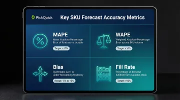
Key forecast accuracy metrics to track:
- MAPE (Mean Absolute Percentage Error): 10–25% is generally strong for FMCG/staples with stable demand; expect 25–35% during promotional periods
- WAPE (Weighted Absolute Percentage Error): Preferred over MAPE for retail portfolios because it avoids small-SKU distortion
- Bias: Consistent over- or under-forecasting indicates systematic model errors
- Fill rate: The operational outcome metric that measures availability
When actual sales deviate significantly from forecast, investigate the cause. It's often a demand driver the model didn't capture—a competitor going out of stock, a viral trend, or a platform push notification campaign. Update model inputs accordingly.
Key Forecasting Methods for SKU-Level Demand
Time Series Methods
Moving averages, exponential smoothing, and ARIMA all rely solely on a SKU's own historical demand record, extracting trend, seasonality, and cyclical signals from past sales.
These methods perform well when:
- SKUs have stable, long sales histories
- Seasonal patterns are predictable
- Promotional interference is minimal
They struggle, however, when applied to:
- New SKUs with sparse history
- Highly promotional or event-driven demand
- Sudden shifts in consumer behavior
Causal / Regression-Based Models
ARIMAX and dynamic regression extend standard time series by incorporating external variables—promotional spend, price changes, competitor activity, and festive calendars. In the M5 retail forecasting competition, ARIMAX (with covariates) was 13% more accurate than standard ARIMA.
These models are best suited for:
- FMCG brands running active promotional cycles
- Demand with strong seasonality tied to festivals such as Navratri or Diwali
- Categories where price elasticity is a primary demand driver
Machine Learning Approaches
Gradient boosting, random forests, and neural networks represent the current performance ceiling for SKU-level forecasting. The top 50 performing methods in the M5 competition beat the most accurate statistical benchmark by more than 14%; the top five exceeded it by more than 20%. LightGBM, a gradient boosting approach, showed the strongest individual performance among ML methods tested.
The trade-off is real, though. ML models offer clear advantages:
- Process large feature sets across many SKUs simultaneously
- Identify non-linear relationships that traditional models miss
- Exploit cross-SKU patterns such as pack-size substitution behavior
But they also come with higher requirements:
- More historical data than classical methods
- Computational resources for training
- Expertise in model tuning and feature engineering
The Clustering-Then-Model Approach
Choosing a single model architecture across hundreds of SKUs ignores the fact that a slow-moving masala variant and a high-velocity dairy SKU behave nothing alike. The clustering approach solves this by grouping SKUs by demand behavior—stable high-velocity, seasonal, slow-moving, intermittent—then building or tuning separate models for each cluster.
The efficiency gains are concrete: a cluster-based selection approach produced forecast values in 6 hours 30 minutes, while random model selection took 15 hours 36 minutes, cutting computational time by more than half while improving accuracy.
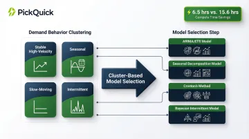
For regional brands managing dozens of variants across Blinkit, Zepto, and Swiggy Instamart simultaneously, this kind of structured segmentation is what keeps forecasting operationally viable at scale.
Factors That Affect SKU Forecast Accuracy in Quick Commerce
Festive and Regional Seasonality
Unlike traditional e-commerce where festive purchases spike weeks before the event, Quick Commerce sales spike on the exact day of the occasion.
Documented demand lifts:
- New Year's Eve 2025 drove order volumes to ~1.4–1.5x of BAU and GMV to ~1.6x of BAU
- Quick commerce orders recorded over 85% growth in volumes during the first week of Diwali festive sales
Regional seasonality matters intensely for masala and staples brands. Wedding season, Navratri, and regional festivals create sharp demand spikes that must be incorporated into forecasting models as explicit calendar variables.
Promotional Events
Festive spikes are predictable — promotional volatility is not. Promotional policies such as giveaways and flash sales are intensively used in e-commerce, significantly affecting sales volume and creating high variance. Traditional statistical models perform adequately in non-promotional periods but falter during high-variance sales events. Machine learning models must explicitly incorporate promotional calendars as covariates to prevent severe MAPE degradation.
Pin-Code-Level Micro-Demand Variations
Demand is traced in real time and at a micro level, sorted by locality, time of day, and consumption behavior. Blinkit plans assortment store by store rather than city-wide, defining what sells in one neighborhood and what may not move at all just a few kilometers away.
Time-of-day variance:
Beverages peak in morning hours driven by tea/coffee routines, while chocolates see upticks post-lunch and late-night driven by cravings.
Data Quality and Recency
Sparse or inconsistent historical data for newer SKUs or recently launched cities makes standard time series approaches unreliable. Proxy data (similar SKU histories, category benchmarks) and shorter-horizon forecasts can partially compensate.
Consolidated platform operations also help here. When replenishment, availability tracking, and Min-Max optimization are managed across Blinkit, Zepto, Swiggy Instamart, and JioMart through a single operator, brands gain richer, unified input data — improving forecast reliability compared to managing each platform independently.
Common Mistakes Brands Make with SKU-Level Forecasting
Using Category-Level Trends for Individual SKU Decisions
The most damaging error: using category-level or brand-aggregate demand trends to make individual SKU replenishment decisions. This causes high-velocity SKUs to run out while slow movers pile up in the dark store.
Category-level forecasts are appropriate for procurement planning and budget allocation. They are dangerously misleading for replenishment execution.
Building a Forecast Model Once and Forgetting It
The miscalibration problem: building a forecast model once and treating it as a permanent solution. In reality, demand patterns for QC shift frequently. Static models degrade in accuracy — and teams rarely notice until stockouts or overstock events surface the gap.
Common triggers for model drift include:
- Platform promotions shifting purchase timing and volume
- Competitor assortment changes pulling demand across SKUs
- Evolving consumer preferences (pack size, format, flavour)
- Seasonal demand spikes not captured in baseline data
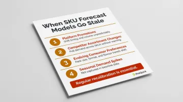
Forecast models naturally become outdated as demand patterns evolve, new products are introduced, and market conditions change. Regular recalibration is essential.
Assuming Offline Demand Mirrors QC Demand
Brands with large GT/MT networks often assume QC demand mirrors offline sales proportionally across pack sizes and flavours. In practice, QC shoppers tend to skew differently.
Example divergence:
- Dairy: A regional brand may see 1-litre packs lead offline, while QC shoppers overwhelmingly prefer 500ml packs for immediate consumption
- Masalas: CTC variants (Chilli, Turmeric, Coriander, Cumin) dominate offline, but blended masalas (Biryani, Chaat, Chole) over-index on QC due to impulse-driven cooking needs
Frequently Asked Questions
What is SKU-level forecasting?
SKU-level forecasting predicts future demand separately for each individual product variant—distinct from category or brand-level forecasts—so that inventory and replenishment decisions reflect the actual demand pattern of each specific item.
What are the 5 types of demand forecasting methods?
The five main families are:
- Time series methods: moving averages, exponential smoothing, ARIMA
- Causal/regression models: ARIMAX and similar approaches
- Machine learning: LightGBM, XGBoost
- Qualitative/judgmental methods: expert input and market intelligence
- Simulation-based models: scenario and Monte Carlo approaches
The right choice depends on your data availability and the nature of your demand pattern.
Can ChatGPT do forecasting?
No. A 2024 NeurIPS study found that removing the LLM component from forecasting pipelines did not degrade performance (results often improved). Purpose-built statistical or ML models trained on structured sales data are required for reliable SKU-level predictions.
What is the difference between SKU-level and category-level forecasting?
Category-level forecasting aggregates demand across all variants, which can mask critical stockout risks in individual SKUs. SKU-level forecasting reveals these hidden imbalances and enables precise replenishment decisions.
How do you forecast demand for new SKUs with no sales history?
Lean on the sales history of similar existing SKUs or apply category-level velocity benchmarks as a starting point. Begin with conservative short-horizon forecasts, then quickly adjust as early sales data comes in. Clustering SKUs by demand behavior can also provide useful proxy signals.
How often should SKU demand forecasts be updated in Quick Commerce?
The fast replenishment cadence of Quick Commerce (QC), often daily or every few days, means forecasts should be refreshed at minimum weekly. Near-real-time updates are ideal whenever significant demand signals occur, such as promotions, platform pushes, or stockout recoveries.