Introduction
Every weekend, a regional masala brand running on Blinkit faces the same operational nightmare: five dark stores in South Bengaluru stock out of their bestselling Sambhar masala by 9 PM, while three dark stores in Pune sit with 40% overstock of the same SKU, blocking shelf capacity for faster-moving variants. Both failures hurt the brand's platform ranking and trigger availability score penalties that take weeks to recover from.
This isn't a logistics problem or a supply chain breakdown. It's a demand visibility problem that starts at the SKU × dark store level. When forecasting happens at the brand or category level, it completely misses the hyperlocal demand patterns that drive Quick Commerce performance. Stockouts hit high-velocity pincodes during peak hours, slow pockets accumulate dead stock, and algorithmic suppression compounds both problems simultaneously.
This guide gives brand managers and QC operators a practical framework for forecasting demand at the SKU and dark store level — covering the methods that work within Quick Commerce's compressed timelines, and how to measure and improve accuracy before a single availability dip triggers platform-wide visibility penalties.
Key Takeaways
- SKU & store level forecasting predicts demand for each individual product at each specific dark store, not at aggregate brand or category level
- Quick Commerce's ultra-short replenishment windows and platform penalties for stockouts make granular forecasting non-negotiable
- Effective forecasting combines historical sales velocity, external signals (promotions, seasonality), and SKU clustering to handle data sparsity
- Tracking MAPE and Bias at the SKU-store level, then feeding those learnings back into the model, is what separates consistently in-stock brands from those that miss fill rate targets
What Is SKU & Store Level Demand Forecasting?
SKU-level forecasting means predicting demand for each individual product unit (by variant, pack size, weight, flavour) independently, rather than rolling up to a category or product family. This granularity matters because two SKUs in the same category can have completely different velocity, seasonality, and regional pull.
A 250g Biryani masala might move 3x faster than a 100g variant in the same dark store. Forecasting them as a single aggregate would systematically under-stock the high-velocity item while over-stocking the slower one.
Store-level (or dark store/pincode-level) forecasting applies that SKU-level forecast to each specific fulfillment node. A 250ml mango lassi may sell 5x faster in a Mumbai dark store than in a Delhi one, driven by regional taste preferences, local competition, and micro-market demand patterns. Aggregated forecasting misses this entirely — you end up stocked out in Mumbai while the same SKU sits unsold in Delhi.
The Demand Hierarchy
Forecasting accuracy improves as you disaggregate, but so does complexity:
- Brand level → High-level visibility, masks local variation
- Category level → Slightly better, still hides SKU-specific patterns
- SKU level → Captures product-specific velocity and seasonality
- SKU × dark store level → Maximum granularity, highest actionability
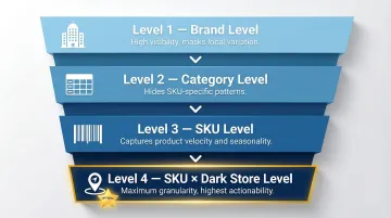
The goal is to find the right level of granularity that your replenishment system can actually act on. For Quick Commerce — where replenishment happens multiple times daily and platforms penalize stockouts algorithmically — SKU × dark store level forecasting is the only approach that matches operational reality.
Why Forecasting at This Level Is Uniquely Challenging for Quick Commerce Brands
Ultra-Short Replenishment Cycles
Unlike general trade or modern trade with weekly or biweekly stock cycles, QC dark stores require replenishment every 1–3 days. This compresses the time available to react to forecast errors. A wrong forecast doesn't just cause inconvenience: it triggers an immediate out-of-stock flag on the platform within hours. According to industry practices, automated Warehouse Management Systems (WMS) monitor dark store stock levels in real-time and trigger replenishment when inventory drops below configured thresholds, operating on intra-day cadences rather than weekly planning cycles.
Platform Visibility Penalties
QC platforms algorithmically suppress SKUs that are frequently out of stock or have low availability scores. Blinkit expects a sustained fill rate above 90%; dropping below 80% consistently triggers algorithmic demotion, reducing search ranking and ad visibility. Running ads while out of stock in a specific dark store yields zero impressions—the inventory must be physically present in the consumer's local dark store to be digitally visible.
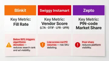
For brands scaling across multiple platforms, the stakes are even higher:
| Platform | Key Metric | Visibility Penalty |
|---|---|---|
| Blinkit | Fill Rate | Below 80% triggers algorithmic demotion; reduces search rank and ad visibility |
| Swiggy Instamart | Vendor Score (LTA, OTIF, LFR, UFR) | Low scores cut Purchase Order volumes and risk SKU delisting |
| Zepto | PIN-code Market Share | Poor share triggers reduced platform visibility; Zepto Atom (₹30,000/month) offers minute-by-minute PIN-code data to address this |
Demand Sparsity at the Tail
At the SKU × dark store intersection, many SKUs show intermittent or sparse sales data—especially for new listings or slower-moving variants. This makes traditional time-series models unreliable. For intermittent demand patterns, specialized methods like the Syntetos-Boylan Approximation (SBA) or Teunter-Syntetos-Babai (TSB) method are required to prevent bias and obsolescence risk. Standard exponential smoothing applied to sparse data results in severe forecast bias.
The starting point is classifying each SKU's demand pattern using the Coefficient of Variation (CoV) framework, which determines which forecasting method applies:
- Smooth demand: ADI < 1.32 and CV² < 0.49 (forecastable using standard methods)
- Intermittent demand: ADI ≥ 1.32 and CV² < 0.49 (requires specialized methods like SBA)
- Lumpy demand: ADI ≥ 1.32 and CV² ≥ 0.49 (highly unforecastable; requires safety-stock-heavy policies)
High Demand Volatility from Promotions and Platform Events
Flash sales, platform-curated offers, and influencer-driven spikes create sudden demand surges that historical averages don't capture. An early onset of summer can push up demand for ice creams and dairy beverages by upwards of 30%. Unlike traditional e-commerce where festive buying peaks days in advance, QC sales spike on the exact day of the occasion—Diwali, Eid, or regional festivals—making promotional calendars a critical forecasting input.
Multi-Node Complexity
That volatility problem compounds at scale. Regional brands running across 10+ cities on 3–4 platforms face a combinatorial explosion of SKU × dark store combinations—and spreadsheet-based tracking breaks down well before you hit 500 combinations. Operators managing hundreds of regional brands across 10,000+ pincodes treat Min-Max optimization and velocity-based replenishment as systematic operating disciplines, built into daily workflow rather than triggered reactively.
Core Demand Forecasting Methods That Work at SKU & Store Level
Time-Series Methods (For SKUs with Sufficient History)
ETS (Exponential Smoothing), ARIMA, and TBATS are well-suited for SKUs with consistent, non-sparse historical velocity. These methods extract trend and seasonality patterns from past sales to project forward.
TBATS handles QC demand with complex, overlapping seasonalities — for example, time-of-day spikes combined with day-of-week patterns. It uses Fourier terms, exponential smoothing, and Box-Cox transformations (a variance-stabilizing technique) to model multiple seasonal periods simultaneously.
Limitation: These methods break down when data is sparse or when external events (promotions, weather, platform sales) drive demand shifts that historical patterns don't capture.
Machine Learning Methods (For SKUs with Rich, Multi-Signal Data)
ML models like gradient boosted trees (XGBoost, LightGBM) consume a wide feature set—lag-based sales features, promotional calendar, day-of-week patterns, pincode demographics, platform ranking data—and identify non-linear relationships that time-series models miss.
In the M5 Forecasting Competition using Walmart retail data, gradient boosted ensemble learners dominated the top rankings, proving particularly effective when the same model is trained across many SKUs simultaneously, allowing cross-learning from correlated demand patterns.
Clustering-Based Approach (For Handling Scale and Sparsity)
Rather than building one model per SKU, group SKUs with similar demand patterns—by velocity, seasonality shape, or category—into clusters, then build a model per cluster. This solves the data sparsity problem for new or low-velocity SKUs by borrowing statistical strength from similar products.
Hierarchical forecast reconciliation using the Minimum Trace Shrinkage estimator (MinT-Shrink) improves accuracy by 1.7% to 3.7% by combining signals across aggregation levels — forecasting at the city or category level, then reconciling down to the store level, lifts accuracy for sparse SKUs.
Before modeling, use Coefficient of Variation (CoV) to assess which SKUs are statistically forecastable and which need a fallback strategy — such as safety stock rules — instead of a full statistical model.
Incorporating External/Exogenous Signals
High-performing QC forecasts consistently layer in external variables:
- Promotion calendars and platform event schedules
- Weather patterns (critical for beverage/dairy categories)
- Local festivals and regional events
- Day-of-week and time-of-day patterns
ARIMAX (AutoRegressive Integrated Moving Average with Explanatory Variables) models are recommended to ingest these exogenous variables. Without these signals, forecasts will systematically under-predict during high-demand events.
Hybrid and Ensemble Approaches
No single method wins universally across hundreds of SKUs and dozens of dark stores. Modern QC forecasting often uses an ensemble—a baseline time-series forecast blended with an ML adjustment for promotional periods.
Whichever ensemble you choose, the validation method is non-negotiable. Use time-series-appropriate contiguous hold-out sets, not random splits. The correct approach is "evaluation on a rolling forecasting origin" (time-series cross-validation) — the training set must consist only of observations prior to the test set, eliminating future data leakage.
Best Practices for SKU & Store Level Demand Forecasting in Quick Commerce
Start with Data Hygiene and a Forecastability Audit
Before building any model, audit your historical sales data at the SKU × dark store level:
- Identify data gaps (OOS periods, listing gaps)
- Clean anomalies and outliers
- Classify SKUs by forecastability using CoV
SKUs with CV² above 0.49 and ADI ≥ 1.32 are lumpy/unforecastable—apply rule-based safety stock approaches rather than statistical forecasting. Don't waste model complexity on unforecastable SKUs.
Segment SKUs by Velocity and Manage Them Differently
Divide your SKU portfolio using ABC-XYZ inventory segmentation:
- Category A (10-20% of items generating 70-80% of revenue): Apply time-series or ML forecasting with tight control and daily monitoring
- Category B (30% of items generating 15-20% of revenue): Use standard forecasting methods with moderate oversight
- Category C (50-60% of items generating 5-10% of revenue): Use simpler Min-Max replenishment rules with looser controls
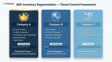
This tiered approach keeps forecasting manageable across a large SKU portfolio. PickQuick's dark store replenishment operations apply Min-Max optimization as part of managing availability metrics across 10,000+ pincodes, using performance-based expansion where Max levels grow only when brands demonstrate zero stockouts, clean motherhub inventory, and strong velocity.
Build Forecast Models at the Right Hierarchy Level and Disaggregate Down
Forecast at a level where you have sufficient data density (for example, brand × city × week). Then disaggregate down to the SKU × dark store level using proportional profiles based on each store's historical sales mix.
This "plan high, source low" approach works particularly well for:
- New listings with limited store-level history
- Sparse SKUs where dark store data is thin
- Regional rollouts where city-level signals are stronger than pincode signals
Anchoring to a stable aggregate signal before splitting down reduces noise and improves accuracy at the edges of your catalog.
Integrate the Promotional and Platform Events Calendar as a First-Class Input
Make promotion planning a formal input to the forecasting process—not an afterthought. Create a structured events calendar capturing:
- Platform sales (Blinkit sales, Zepto flash promotions)
- Festive periods (Diwali, Eid, regional festivals)
- App-exclusive offers
- Seasonal demand drivers (weather, harvest seasons)
Incorporate multipliers or dummy variables for these periods into your models. Brands that treat promotions as unexpected spikes and adjust forecasts in advance consistently outperform those reacting after the fact.
Close the Feedback Loop
Compare forecast vs. actuals at the SKU × dark store level weekly. Track:
- Bias: Are you systematically over- or under-forecasting certain SKUs or dark stores?
- MAPE: What is the absolute percentage error?
Feed these error diagnostics back into model recalibration. A weekly review cadence—reviewing bias and MAPE together—catches drift early, before it compounds into stockouts or excess inventory at specific dark stores.
How to Measure and Continuously Improve Forecast Accuracy
Key Metrics to Track
MAPE (Mean Absolute Percentage Error) measures overall forecast accuracy. For Consumer Packaged Goods (CPG), a MAPE of 15%–25% is generally considered acceptable, with high-velocity items typically achieving lower error.
At the SKU × dark store level for QC, a target MAPE under 20–25% for high-velocity SKUs is strong performance. Sparser SKUs will naturally carry higher error and should be managed with buffer stock rather than optimized solely for MAPE.
Forecast Bias identifies systematic over- or under-prediction. Bias occurs when there is a consistent difference between actual sales and the forecast. Positive bias means chronic over-forecasting (leading to excess inventory and ageing); negative bias means chronic under-forecasting (leading to stockouts and availability penalties).
Caution: MAPE is heavily distorted by intermittent demand (where actual sales are zero), making it a misleading metric for slow-moving SKUs at the dark-store level. Use weighted MAPE or alternative metrics for C-tier SKUs.
Monitor Availability Metrics as a Proxy for Forecast Quality
On QC platforms, In-Stock Rate and Fill Rate at the dark store level directly reflect forecast accuracy. Watch for these common signals of systematic under-estimation:
- Availability drops consistently on weekends or post-promotion windows
- Fill rate declines on specific SKUs after a platform-run offer
- In-stock gaps cluster around the same dark stores repeatedly
These metrics make forecast performance tangible — they tie directly to revenue and platform ranking. If a product is unavailable, 50% of consumers will switch to another QC platform, making availability the most consequential measure of forecasting success.
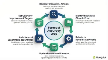
Continuous Improvement Cycle
When availability signals flag a problem, the response needs structure. Establish a regular cadence (weekly or biweekly) to:
- Review forecast vs. actuals at the SKU × dark store level
- Identify SKUs with chronic error
- Retrain or recalibrate models
- Update the promotional calendar with learnings
- Build internal benchmarks for each SKU tier
- Set improvement targets quarter over quarter
Track MAPE trend, bias direction, and availability metrics together — not in isolation. If all three are improving quarter over quarter, your forecasting system is compounding its accuracy. If MAPE holds steady but availability keeps slipping, the issue is likely execution gaps at the dark store level, not the model itself.
Frequently Asked Questions
What are the steps for successful demand planning and replenishment?
Gather clean historical data at the SKU × dark store level, choose the right forecasting method per SKU tier (time-series for high-velocity, safety stock for intermittent), generate a forecast incorporating promotional signals, translate it into a replenishment plan, execute the restock, then compare actuals to forecast and refine weekly.
What is SKU level forecasting?
SKU-level forecasting generates individual demand predictions for each product variant—by size, flavour, or pack size—rather than at an aggregate category or brand level. This prevents over-stocking slow movers while ensuring high-velocity items stay available.
What are the main demand forecasting methods?
The main categories are time-series methods (ARIMA, ETS, TBATS for seasonal patterns), machine learning methods (gradient boosting, regression for multi-signal data), and specialized intermittent demand methods (SBA, TSB). The best approach depends on data availability, SKU characteristics, and demand predictability.
How can historical data help in SKU-level demand forecasting?
Historical sales data reveals velocity, trend, and seasonality per SKU, forming the baseline for all statistical models. It also enables proportional profiling—using similar product histories to generate forecasts for new or sparse SKUs where direct data is thin.
What is a good demand forecast accuracy?
For Quick Commerce at the SKU × dark store level, under 25% MAPE for A-tier SKUs is strong performance; C-tier SKUs need safety stock strategies rather than MAPE optimization. Broadly, 15%–25% MAPE is considered acceptable for FMCG SKU-level forecasting, with high-velocity items typically achieving the lower end.
What is the golden rule of forecasting?
The golden rule: all forecasts are wrong. The goal is to make them less wrong over time. This means structured feedback loops, continuous recalibration, and using forecast error diagnostics to improve future models rather than treating any forecast as a fixed output.